Understanding The Internals Of Rag
In a previous blog post, I detailed a possible technical setup for having a solid foundation for doing RAG within the Springboot ecosystem, using docker to leverage locally downloaded LLMs and Postgres, configured with the PGVector extension to be able to manipulate and store embeddings and work with similarity search from a Postgres DB. If you haven’t yet, go read that one, as it will greatly help with digesting this upcoming content, even if I’ll try to make this as self-contained as possible.
Recap - what are embeddings after all?
Note the below two paragraphs are adapted from the awesome Ollama blog, credits go to them! Emphasis mine.
At a very broad level, embedding models are models that are trained specifically to generate vector embeddings: long arrays of numbers that represent semantic meaning for a given sequence of text:
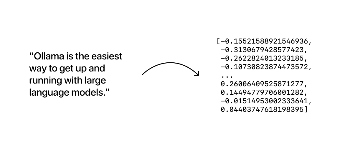
The resulting vector embedding arrays can then be stored in a database, which will enable us to compare them as a way to search for data that is similar in meaning.
What this means is that, essentially, we perform a domain transform: just like the Fourier Transform can map a signal from the time to the frequency domain, we are mapping long sequences of text into a “vector-domain”, producing an alternative representation of the text. The main insight is that in this new “vector domain”, it is simpler and easier to search for “similar enough” texts in a way that plain text doesn’t allow us to.
The shift from the text domain to the vector domain needs to encode the semantic meaning of the text in some way, which is the aspect that makes this work: it’s not only a matter of applying a simple change from words to vectors, but, it’s really about capturing the semantic meaning of the text. Embedding models are, generally neural network algorithms that can be thought of as a checkpoint step in an LLM completion generation flow, that generates embeddings when an input is provided and stop there.
Current LLM providers like OpenAI, AWS Bedrock, Anthropic, and several other open-source projects, offer two distinct APIs: firstly, what is called an inference API, which is what is known colloquially as a large language model: text goes in, in the form of a prompt, and a completion, usually in the form of human-readable text, an image, a video or even audio, comes out. Secondly, an embeddings API, which is an API whose sole responsibility is to produce embeddings from a piece of text and is arguably, the most important step in a deployed, trained, and fine-tuned LLM request flow.
Embeddings are the crucial piece of the puzzle for understanding RAG.
Requirements for embeddings to work
Another crucial point to understand is that each provider offers different embedding models that support different context window sizes (the size, measured in tokens, of the largest chunk of text you can embed at once) as well as different dimension sizes (the number of dimensions, i.e. elements, in the “vector-representation” of the embedded text). These two numbers mean different things and play different roles at different levels of the stack. Online, the most looked-at numbers you’ll often read about concern only the number of elements in the “vector-representation” of the text, so, when you read online that “OpenAI embeddings have 1536 dimensions” or that “the default embedding size of PGVectorStore is set to 1536”, this just means that the number of elements of the vectors that encode the semantic meaning of the text is 1536. There are many different models, from open-source to proprietary that have different dimensions, from 768 dimensions to over 3000, the flavors are quite varied here, and, a lot of the work is in testing the different trade-offs between different sizes in terms of how well the embeddings perform across a range of aspects, from size taken in the DB tables where they are stored, to the performance of using them with different distance types (we’ll see what these are later).
So, what is the most important aspect when working with embeddings? Very simply, and also obviously, the embeddings of potential documents meant to be used for RAG purposes need to be done by the same model that will embed the query for optimal results. If the vectors would have different sizes, applying a distance metric to them wouldn’t make sense. Obviously what this also means is that in theory different embedding models that produce vectors of similar sizes could be used, the results would be meaningless to interpret as the representations in semantic meaning would be different, even if the size of the resulting vectors would be the same. Just because we can, doesn’t mean we should.
Back to Springboot: how does this work in practice?
Now that we’ve seen some of the theory, let’s look at some code to make it more concrete.
Springboot has a new module, Spring AI, which we can leverage to integrate embeddings (and a dedicated database to work with them) into a regular Springboot web application.
Just like there are many distinct Large Language Models and Embedding providers, we can have many distinct “vector database” providers.
In the remainder of this post, I’ll focus on integrating only open-source variants of all we’ve been discussing so far:
- LLMs are stored and run locally, via the Ollama project, packaged as a docker container;
- Postgres will serve as our vector store, by being extended with the
PGVectorextension; - The embedding model to be used will be mxbai-embed-large-v1 from Mixedbread;
All of this has been written in the previous blog post, but, in the interest of making this post fully self-contained, I’ll extract the key pieces and repeat them here for reference.
Ollama is a cool new project that surfaced as a way to leverage the power of LLMs and embedding models by allowing people to run them locally on their machines. The base docker setup I used (as part of a larger docker-compose file that instantiated more services, such as the Springboot application and a Streamlit front-end) for setting up Ollama was the following:
  ollama-llm:
    image: ollama/ollama:latest
    volumes:
      - ollama_data:/root/.ollama
    ports:
      - "11434:11434"
    networks:
      - app-network

...

  prepare-models:
    image: ollama/ollama:latest
    depends_on:
      - ollama-llm
    volumes:
      - ollama_data:/root/.ollama
    environment:
      - OLLAMA_HOST=http://ollama-llm:11434
    networks:
      - app-network
    entrypoint: >
      sh -c "
        echo 'Waiting for Ollama server to start...' &&
        sleep 10 &&
        echo 'Pulling tinydolphin...' &&
        ollama pull tinydolphin &&
        echo 'Pulling tinyllama...' &&
        ollama pull tinyllama &&
      echo 'Pulling llama3.1...' &&
      ollama pull llama3.1 &&
      echo 'Pulling embedding model...' &&
      ollama pull mxbai-embed-large &&
        echo 'Model preparation complete.'"

networks:
 - app-network
Ollama, upon start, spins up a server that we can then pull several open-source LLM and embedding models from, so, we do this in a two-image fashion: one that “prepares the models” by pulling them into our machine, into the volume defined by ollama_data, that is then shared with the ollama-llm compose service which will be the actual “running service” that we can then connect to from our Java code, to “call the LLM” as well as for generating the embeddings.
The way this would work in a real production setting would be that the Java Springboot app would have a URL to connect itself to an LLM provider, which, in our case will be the Ollama “self-hosted” model.
Let’s see how this works:
  backend:
    build: .
    ports:
      - "8080:8080"
    environment:
      - SPRING_DATASOURCE_URL=jdbc:postgresql://db:5432/ragdb
      - SPRING_DATASOURCE_USERNAME=postgres
      - SPRING_DATASOURCE_PASSWORD=password
      - SPRING_AI_OLLAMA_BASE_URL=http://ollama-llm:11434/
      - SPRING_AI_OLLAMA_CHAT_OPTIONS_MODEL=tinydolphin
      - SPRING_AI_OLLAMA_CHAT_OPTIONS_ALTERNATIVE_MODEL=tinyllama
      - SPRING_AI_OLLAMA_CHAT_OPTIONS_ALTERNATIVE_SECOND_MODEL=llama3.1
      - SPRING_AI_OLLAMA_EMBEDDING_OPTIONS_MODEL=mxbai-embed-large
      - SPRING_AI_VECTORSTORE_PGVECTOR_REMOVE_EXISTING_VECTOR_STORE_TABLE=true
      - SPRING_AI_VECTORSTORE_PGVECTOR_INDEX_TYPE=HNSW
      - SPRING_AI_VECTORSTORE_PGVECTOR_DISTANCE_TYPE=COSINE_DISTANCE
      - SPRING_AI_VECTORSTORE_PGVECTOR_DIMENSIONS=1024
    depends_on:
      - prepare-models
      - db
    volumes:
      - ollama_data:/root/.ollama
    networks:
      - app-network
The key properties for this sub-section are:
- SPRING_AI_OLLAMA_BASE_URL=http://ollama-llm:11434/
- SPRING_AI_OLLAMA_CHAT_OPTIONS_MODEL=tinydolphin
- SPRING_AI_OLLAMA_CHAT_OPTIONS_ALTERNATIVE_MODEL=tinyllama
- SPRING_AI_OLLAMA_CHAT_OPTIONS_ALTERNATIVE_SECOND_MODEL=llama3.1
- SPRING_AI_OLLAMA_EMBEDDING_OPTIONS_MODEL=mxbai-embed-large
We connect to the Ollama running server and configure the models we have downloaded to connect our Springboot app to them.
Let’s now look at how generating embeddings work using the configured model we just downloaded into our Ollama volume.
Generating embeddings in code with mxbai-embed-large-v1
The basic endpoint we’ll use is:
@PostMapping("/query-embedding")
    public String embedding(@RequestBody String query) {
        return embeddingService.computeEmbedding(query).toString();
    }
Inside the EmbeddingService we have:
@Slf4j
@Service
@AllArgsConstructor
@ConditionalOnProperty("spring.datasource.url")
public class EmbeddingService {

    @Qualifier("ollamaEmbeddingModel")
    private EmbeddingModel embeddingModel;

    public List<Double> computeEmbedding(String query) {
        return embeddingModel.embed(query);
    }
...
}
The real link between this piece of code and the docker-compose configuration shown above is “tucked away” in the Qualifier annotation, as we see upon “following” the qualifier declaration:
 @Bean
    @ConditionalOnMissingBean
    @ConditionalOnProperty(
        prefix = "spring.ai.ollama.embedding",
        name = {"enabled"},
        havingValue = "true",
        matchIfMissing = true
    )
    public OllamaEmbeddingModel ollamaEmbeddingModel(OllamaApi ollamaApi, OllamaEmbeddingProperties properties) {
        return new OllamaEmbeddingModel(ollamaApi, properties.getOptions());
    }
So, by qualifying the EmbeddingModel interface with the annotation, what this means is that Springboot, at runtime will “resolve” to the implementation seen above, and as a result, we will be able to compute embeddings based on the model we defined earlier:
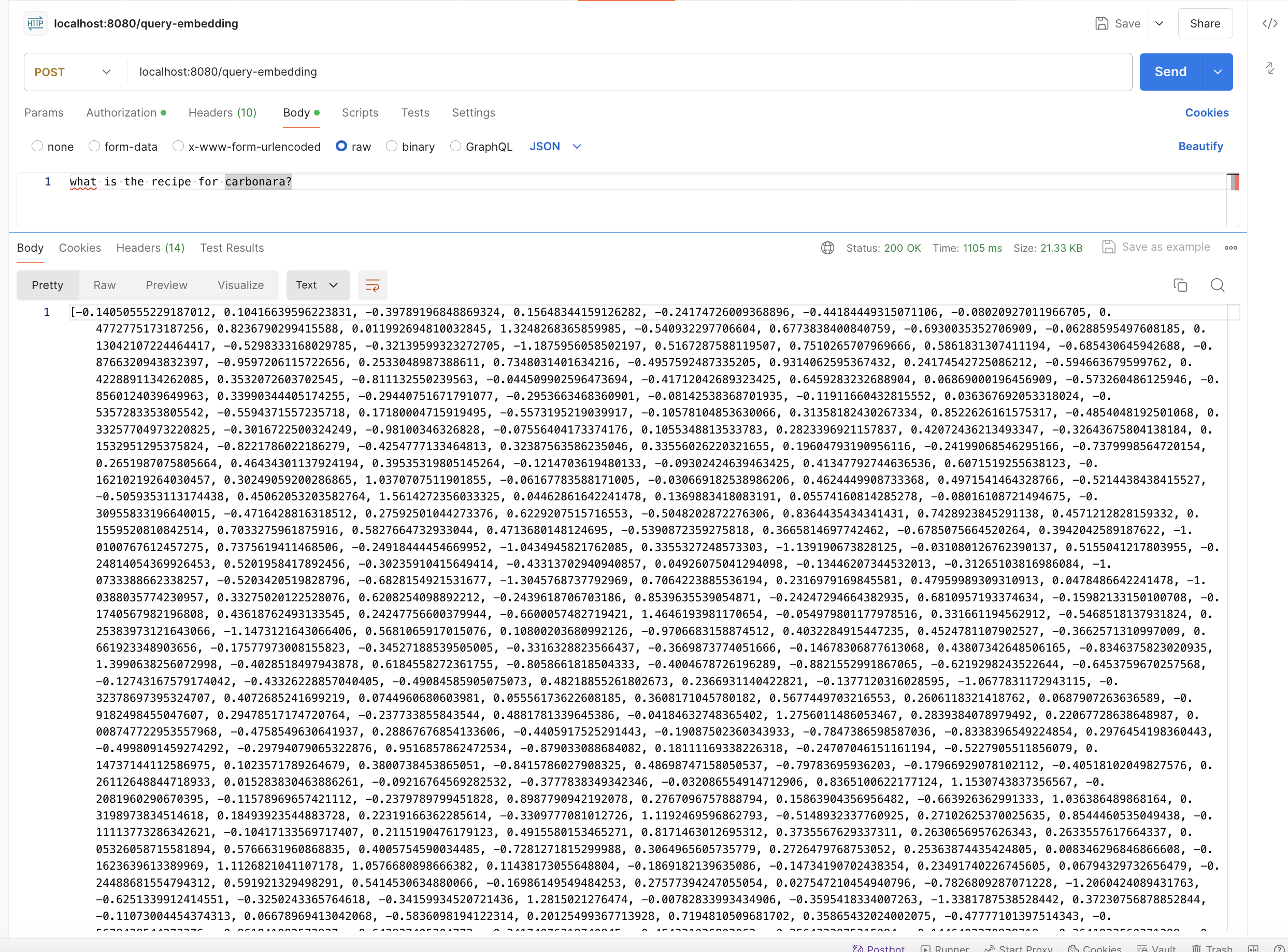
Now we have a vector that captures the “semantic meaning” of our question, which means that these 1024 entries will somehow capture that we are asking for a cooking recipe, and that it’s for pasta carbonara. Remember, we are working with vectors with 1024 elements and we will compare them by default according to the cosine distance “distance type”:
 - SPRING_AI_VECTORSTORE_PGVECTOR_DISTANCE_TYPE=COSINE_DISTANCE
 - SPRING_AI_VECTORSTORE_PGVECTOR_DIMENSIONS=1024
The grand finale: We know how to generate embeddings, now we can compute similarity between texts right inside the DB
Now for the grand finale, we will see how to calculate similarity thresholds right inside the database, leveraging PGVector and what we just learned about embeddings.
We saw earlier that we are using as our “distance type” what is known as “Cosine distance”. What is this distance and how does it relate to the actual “similarity” which is the concept usually exposed in libraries, for example, the Spring AI library:
Fluent expression exposed by the Spring AI library:
 var similarDocuments = vectorStore.similaritySearch(SearchRequest.query(question)
                .withSimilarityThreshold(0.70);
See here, where it says: similarity threshold.
That is defined as the complement of the cosine distance, i.e. if the cosine distance between V1 and V2 is defined as CosineDistance(V1, V2), then we have:
SimilarityThreshold = 1 - CosineDistance(V1, V2)
If we think geometrically, imagine two vectors in the XY cartesian plane, and imagine both vectors have the same origin point, and now, imagine an angle between them.
The smaller the angle between them is, the closer they are to each other, i.e. the more similar they are. In the limit, when the angle between the vectors is 0, the cosine similarity is 1, and the cosine distance is 0, i.e. there is NO DIFFERENCE between the vectors, so, they are exactly the same.
This is also why the dimensions need to be the same for the embedded documents and question: the difference in the length of the vectors would mess up the calculations!
Note also that, given the definitions of these concepts, cosine distance ranges from 0 to 2, where 0 means identical vectors and 2 means opposite vectors. Correspondingly, cosine similarity ranges from 1 (identical) to -1 (opposite).
Let’s setup a basic table in the DB:
root@b5a235d77c0b:/# psql -U postgres -d ragdb
psql (15.4 (Debian 15.4-2.pgdg120+1))
Type "help" for help.

ragdb=# -- Create a table to store our vectors
CREATE TABLE IF NOT EXISTS vector_examples (
    id SERIAL PRIMARY KEY,
    description TEXT,
    embedding vector(1024)
);
CREATE TABLE
ragdb=#
Now, let’s keep the same example as before:
Let’s assume the question we ask is:
“what is the recipe for carbonara?”
This generates an embedding:
[-0.14050555229187012, 0.10416639596223831, -0.39789196848869324, 0.15648344159126282, -0.24174726009368896, -0.44184449315071106, -0.08020927011966705, 0.4772775173187256, 0.8236790299415588, … (rest ommited), -0.24939970672130585, 0.6905518174171448, 0.6164807081222534]
Let’s now create two separate embeddings and enter them in the DB: one will be an answer to the question and the other will be a short sentence on why Verstappen is the best driver since Schumacher.
ragdb=# INSERT INTO vector_examples (description, embedding) VALUES
('To cook carbonara, mix eggs with parmesan, add guanciale, reserve pasta water, boil pasta, combine in a pan and enjoy!', '[-0.10348883271217346, 1.0759119987487793, 0.048883289098739624, -0.09129567444324493, -0.45658212900161743, -0.019695669412612915, 0.23682862520217896, 0.49972328543663025, 1.073593020439148, 0.2860829532146454, 1.6310596466064453, .... 0.6900556087493896, 0.2374967336654663]);
INSERT 0 1

ragdb=# INSERT INTO vector_examples (description, embedding) VALUES
('Verstappen is a dutch F1 driver who is ruthless on track, and drives the iconic RB20, beating greats like Schumacher and Senna!', '[-0.5480663776397705, 0.011026214808225632, -0.21971482038497925, 0.2039300948381424,, ....  -0.0753195732831955, 0.12138164043426514]);
INSERT 0 1
Now, we are ready to apply the calculation of the cosine similarity:
We see, by consulting the PGVector documentation that such a distance type is represented by the <=> operator in postgres, so, our query will be:
SELECT description, embedding <=> '<the vector that represents the embedding of our question on how to cook carbonara> as cosine_distance FROM vector_examples ORDER BY cosine_distance ASC`
We get:
                                                          description                                                           |  cosine_distance
---------------------------------------------------------------------------------------------------------------------------------+--------------------
 To cook carbonara, mix eggs with parmesan, add guanciale, reserve pasta water, boil pasta, combine in a pan and enjoy!          | 0.1745348873407664
 Verstappen is a dutch F1 driver who is ruthless on track, and drives the iconic RB20, beating greats like Schumacher and Senna! | 0.6636126533319713
As we expected based on the definitions we introduced above, the entry that better matches our query, i.e. the “closest”, has a smaller value for the cosine_distance. Why? Because, mathematically, the vectors are “closer together”, so their cosine_distance is smaller.
The similarity is the complement of this:
                                                           description                                                           |  cosine_distance   |     similarity
---------------------------------------------------------------------------------------------------------------------------------+--------------------+--------------------
 To cook carbonara, mix eggs with parmesan, add guanciale, reserve pasta water, boil pasta, combine in a pan and enjoy!          | 0.1745348873407664 | 0.8254651126592336
 Verstappen is a dutch F1 driver who is ruthless on track, and drives the iconic RB20, beating greats like Schumacher and Senna! | 0.6636126533319713 | 0.3363873466680287
So, we now see that the first value is more similar to our query in the embedding space which is exactly what we wanted to confirm!!
Armed with this, hopefully, you’ll be in a better position to understand how to extract the most out of your RAG workflows! It’s all Math!!